Exercises 10 - Bar Plots

We’ll continue to work on the same .Rmd file from the previous exercise.

---

1. Filter the data by the names of interest we have, group the data by name, and find the total counts using the code below:

names <- c("Justin", "George", "Alexander", "Jacob", "Anderson")
barData <- BabyNamesFull %>%
  filter(name %in% names) %>% 
  group_by(name) %>%
  summarise(total = sum(count))

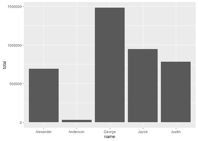
1. Use the data object created to create a bar plot with names on the x-axis and the total count on the y-axis. You’ll need to specify both the x and y variables and change the statistic to “identity” in the geom_bar() function.

ggplot(barData) +
  geom_bar(stat = "identity", aes(x = name, y = total)) 

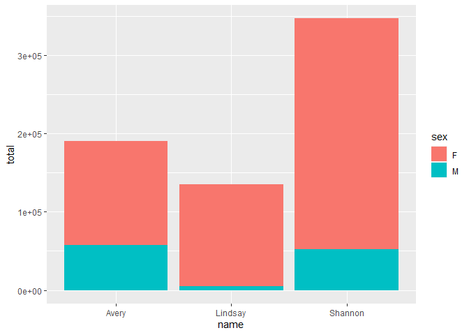
1. Use the data object created by the code below to create a filled bar plot with the sex variable denoting the coloring of columns.

barDataSex <- BabyNamesFull %>%
  filter(name %in% c("Shannon", "Lindsay", "Avery")) %>% 
  group_by(name, sex) %>%
  summarise(total = sum(count))

## `summarise()` has grouped output by 'name'. You can override using the `.groups` argument.

ggplot(barDataSex) +
 geom_bar(stat = "identity", aes(x = name, y = total, fill = sex)) 

---