What’s in a Name?? (Part 5 Solutions)

Matthew Beckman & Justin Post June 25, 2021

Here, we join an analysis already in progress…

Part 1 (RStudio IDE Scavenger Hunt) has been omitted from the following analysis.
Part 2 (Import Data), Part 3 (R Markdown), and Part 4 (Data Wrangling) have been blended for the purposes of our investigation
Part 5 Exercises Follow

Names to be investigated

We’re investigating the popularity of names in the US each year. Matt has chosen to investigate the names of each person in his immediate family: Matthew, Sarah, Eden, Jack, and Hazel. They’re his favorite people, and also his favorite names! He’s feeling torn about how to include his son Jack in the analysis. Jack’s legal name is “Jon” but he is nearly always called “Jack”–the spelling of “Jon” honors Scandinavian heritage on both sides of the family, and the nickname “Jack” specifically honors his great-grandfather.

Some famous persons by each name of the family include:

Sarah Jessica Parker
Eden Hazard
Jack (Jackie) Robinson
Hazel Findlay
Richard Stallman. Seriously, the first hit of an Internet search for “famous Matthew” was Richard Stallman (!) whose given name is… Matthew. “Matthew the Apostle” (Matt’s namesake) was third on that particular list: https://playback.fm/people/first-name/matthew

This document was last modified 2021-06-25 10:30:13.

Summaries of Name Popularity

According to US Social Security data from 1880 through 2020, “Matthew” was the most frequently occurring name in the family.

# vector of names
beckmans <- c("Matthew", "Sarah", "Eden", "Jack", "Hazel")

BabyNamesFull %>%
    filter(name %in% beckmans) %>%                   
    group_by(name) %>%                               
    summarise(total = sum(count, na.rm = TRUE)) %>%  
    arrange(desc(total))

## `summarise()` ungrouping output (override with `.groups` argument)

We also learned that “Eden” was more balanced between the two sexes when compared to the other names in the family.

BabyNamesFull %>%
    filter(name %in% beckmans) %>%
    group_by(name, sex) %>%                          # Task 4.2.3
    summarise(total = sum(count, na.rm = TRUE)) %>%  # Task 4.2.3
    arrange(name)

## `summarise()` regrouping output by 'name' (override with `.groups` argument)

Matt joined Penn State University in 2015, and coincidentally his son Jack was born earlier that year. Interestingly, the name “Jack” was more popular than “Sarah” in 2015, despite the fact that “Sarah” had been far more common when all years had been combined. Perhaps more surprisingly, the name “Hazel” was nearly as common as “Sarah” in that year!

BabyNamesFull %>%
    filter(name %in% beckmans, year == 2015) %>%
    group_by(name) %>%
    summarise(total = sum(count, na.rm = TRUE)) %>% 
    arrange(desc(total))

## `summarise()` ungrouping output (override with `.groups` argument)

BabyNamesFull %>%
    filter(name %in% beckmans, year == 2015) %>%
    group_by(name, sex) %>%
    summarise(total = sum(count, na.rm = TRUE)) %>% 
    arrange(name)

## `summarise()` regrouping output by 'name' (override with `.groups` argument)

Part 5. Graph it

We want to create a graph that highlights the change in popularity among the names you have chosen over the years.

Task 1: sketch (by hand) the plot you plan to make
- note which variables are aligned to various aesthetics of your plot
- does your plot include multiple layers?
Task 2: is your data set aligned to the intended features of this plot?
- do you need to summarise or mutate the data before creating the plot you have in mind?
- do you need to filter the data to show a desired subset, or will all rows of the data be included?
- when data are aligned to the needs of your plot, we sometimes call this a “glyph-ready” data set
Task 3: run esquisse::esquisser(GlyphReadyDataSet) to draft a plot
- esquisser( ) allows you to prototype various plot features, and then view the corresponding ggplot2 code for your plot
- When you are satisfied, copy the R code and paste into Rmd code chunk
- run the R code chunk to reproduce your plot in R Markdown
- modifiy the plot code as needed to better align with the plot you intend (i.e., the one you sketched by hand).
- ideally, you’ll soon skip the esquisser( ) step as you get moer comfortable with the ggplot2 framework
Task 4: clean up axis labels, add a title, etc if you have not already done so.
Task 5 (Challenge): add a layer to somehow display overall birth trend for context
Task 6 (Challenge): plot the trend for each name as a relative frequency, rather than raw counts

Solution

#library(esquisse)

# Task 5.1 My sketch was a line chart of name popularity over time 
# variable mapping:
#    x-position: year
#    y-position: frequency
#    line color: name

# Task 5.2
BeckmanNamesLine <- 
    BabyNamesFull %>%
    filter(name %in% beckmans) %>%
    group_by(name, year) %>%
    summarise(total = sum(count))

## `summarise()` regrouping output by 'name' (override with `.groups` argument)

# Task 5.3 
# esquisse::esquisser(BeckmanNamesLine)
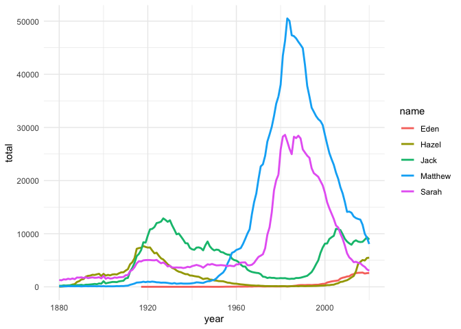
ggplot(BeckmanNamesLine) +
 aes(x = year, y = total, colour = name) +
 geom_line(size = 1L) +
 scale_color_hue() +
 theme_minimal() 

# Task 5.4
TotalBabies <- 
    BabyNamesFull %>%
    group_by(year) %>%
    summarise(totalBorn = sum(count, na.rm = TRUE))

## `summarise()` ungrouping output (override with `.groups` argument)

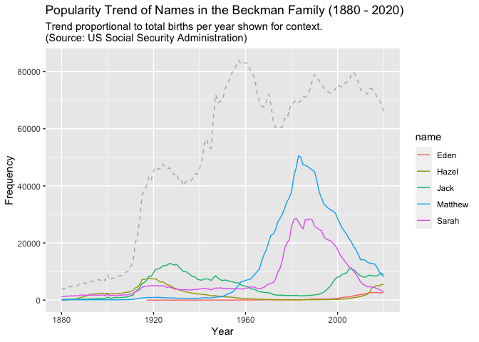
# Task 5.5 (Challenge)
# add context propotional to total births each year to the plot
ggplot(BeckmanNamesLine) +
    geom_line(aes(x = year, y = total, colour = name)) +
    geom_line(data = TotalBabies, aes(x = year, y = totalBorn * 0.02), 
              linetype = "dashed", alpha = 0.3, ) + 
    ggtitle(label = "Popularity Trend of Names in the Beckman Family (1880 - 2020)", 
            subtitle = "Trend proportional to total births per year shown for context.\n(Source: US Social Security Administration)") + 
    ylab("Frequency") + 
    xlab("Year")

# Task 5.6 (Challenge) 
BeckmanNamesRF <- 
    BabyNamesFull %>%
    group_by(year) %>%                    # groups for subsequent mutate()
    mutate(annualTotal = sum(count)) %>%  # new column for yearly totals
    ungroup() %>%                         
    filter(name %in% beckmans) %>%
    group_by(name, year) %>%              # new groups for subsequent summarise()
    summarise(prop = sum(count) / annualTotal)

## `summarise()` regrouping output by 'name', 'year' (override with `.groups` argument)

ggplot(BeckmanNamesRF) +
    geom_line(aes(x = year, y = prop, colour = name)) +
    ggtitle(label = "Popularity Trend of Names in the Beckman Family (1880 - 2020)", 
            subtitle = "(Source: US Social Security Administration)") + 
    ylab("Relative Proportion") + 
    xlab("Year")