Base R Data Structures: Vectors

Common Data Structures

A data scientist needs to deal with data! We need to have a firm foundation in the ways that we can store our data in R. This section goes through the most commonly used ‘built-in’ R objects that we’ll use.

• There are five major data structures used in R

  1. Atomic Vector (1d)
  2. Matrix (2d)
  3. Array (nd)
  4. Data Frame (2d)
  5. List (1d)

Dimension	Homogeneous (elements all the same)	Heterogeneous (elements may differ)
1d	Atomic Vector	List
2d	Matrix	Data Frame
nd	Array

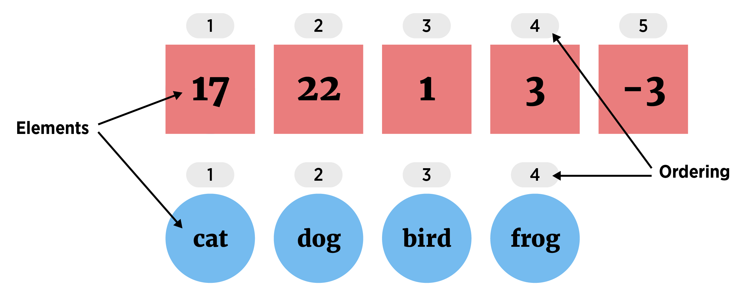
(Atomic) Vector

(Atomic) Vector (1D group of elements with an ordering that starts at 1)

• Elements must be same the same ‘type’ (homogeneous). The most common types of data are:

  • logical, integer, double, and character

Creating a Vector

Many functions output a vector but the most common way to create one yourself is to use the c() function.

• c() “combines” values together
  • Simply separate the values with a comma

#vectors (1 dimensional) objects
#all elements of the same 'type'
x <- c(1, 3, 10, -20, sqrt(2))
x

[1]   1.000000   3.000000  10.000000 -20.000000   1.414214

• Recall the str() function to investigate the structure of the object

str(x)

 num [1:5] 1 3 10 -20 1.41

• The typeof() function tells us which type of data is stored in the vector

typeof(x)

[1] "double"

• Let’s create another vector y with strings stored in it

y <- c("cat", "dog", "bird", "floor")
y

[1] "cat"   "dog"   "bird"  "floor"

str(y)

 chr [1:4] "cat" "dog" "bird" "floor"

typeof(y)

[1] "character"

• We can combine two vectors together using c() as well!

z <- c(x, y)
z

[1] "1"               "3"               "10"              "-20"            
[5] "1.4142135623731" "cat"             "dog"             "bird"           
[9] "floor"          

str(z)

 chr [1:9] "1" "3" "10" "-20" "1.4142135623731" "cat" "dog" "bird" "floor"

typeof(z)

[1] "character"

Notice that R coerces the elements to the data type of the more flexible elements (character - R knows how to convert a number to a character string but doesn’t know how to convert a character string to a number). No warning is produced or message!

You’ll need to get used to how R does these kinds of things implicitly. Check out how R does coercion on some other types of data.

c(TRUE, "hat", 3)

[1] "TRUE" "hat"  "3"   

c(c(TRUE, 3), "hat")

[1] "1"   "3"   "hat"

Notice that the order of operations above is important to understand! In the first line, R coerces the three elements together (character as it is the most flexible). In the second line, R first coerces TRUE and 3 together. TRUE values are treated as 1 (FALSE values as 0). Then the values of 1 and 3 are coerced to character strings to create the final vector.

• One really useful function that creates a vector is the seq() (or sequence) function

seq(from = 1, to = 10, by = 2)

[1] 1 3 5 7 9

seq(1, 10, 1)

 [1]  1  2  3  4  5  6  7  8  9 10

seq(1, 10, length = 5)

[1]  1.00  3.25  5.50  7.75 10.00

• A shorthand for the seq() function is to use a :

1:10

 [1]  1  2  3  4  5  6  7  8  9 10

• This can easily be modified to get other sequences.

20:30/2

 [1] 10.0 10.5 11.0 11.5 12.0 12.5 13.0 13.5 14.0 14.5 15.0

1:15*3

 [1]  3  6  9 12 15 18 21 24 27 30 33 36 39 42 45

Note that R is doing element-wise math. This is the default behavior of doing math on our common data structures (not just vectors!)

• Another function that creates a vector is the runif() (random uniform number generator) function.

runif(4, min = 0, max = 1)

[1] 0.1483719 0.6110159 0.5349631 0.7007864

runif(10)

 [1] 0.33663054 0.54252097 0.38418347 0.22157093 0.08927214 0.32019863
 [7] 0.28526341 0.08016857 0.31166932 0.54710246

runif(5, 20, 30)

[1] 26.70329 25.09878 24.64433 26.93123 28.38150

We’ll find this function really useful when we simulate different quantities!

You might find the different ways to call a function confusing right now! We’ll talk about how to use the help files to understand function calls shortly!

Vector Attributes

R objects can have attributes associated with them. The main attribute that a vector might have associated with it are names for the elements.

u <- c("a" = 1, "b" = 2, "c" = 3)
u

a b c 
1 2 3 

attributes(u)

$names
[1] "a" "b" "c"

There is a special function for getting at the names of an R object. It is the names() function (nice choice there).

names(u)

[1] "a" "b" "c"

Names can be useful when it comes to subsetting and matching observations.

Accessing Elements of a Vector

When thinking about accessing (or subsetting) a vector’s elements, remember that vectors are 1D. We can place the numbers corresponding to the positions of the elements we want inside of [] at the end of the vector to return them. Note: R starts its counting at 1, not 0 like many other languages.

• Return vector elements using square brackets [] at the end of a vector.

letters #built-in vector

 [1] "a" "b" "c" "d" "e" "f" "g" "h" "i" "j" "k" "l" "m" "n" "o" "p" "q" "r" "s"
[20] "t" "u" "v" "w" "x" "y" "z"

letters[1] #R starts counting at 1!

[1] "a"

letters[26]

[1] "z"

• Can ‘feed’ in a vector of indices to []

letters[1:4]

[1] "a" "b" "c" "d"

letters[c(5, 10, 15, 20, 25)]

[1] "e" "j" "o" "t" "y"

x <- c(1, 2, 5)
letters[x]

[1] "a" "b" "e"

We’d call x above an indexing vector

• Use negative indices to return a vector without certain elements

letters[-(1:4)]

 [1] "e" "f" "g" "h" "i" "j" "k" "l" "m" "n" "o" "p" "q" "r" "s" "t" "u" "v" "w"
[20] "x" "y" "z"

x <- c(1, 2, 5)
letters[-x]

 [1] "c" "d" "f" "g" "h" "i" "j" "k" "l" "m" "n" "o" "p" "q" "r" "s" "t" "u" "v"
[20] "w" "x" "y" "z"

• If we have a names attribute associated, we can use names to access elements.

u

a b c 
1 2 3 

u["a"]

a 
1 

t <- c("a", "c")
u[t]

a c 
1 3 

Quick R Video

Let’s look at a quick example of creating and modifying R vectors.

Please pop this video out and watch it in the full panopto player!

• Link to repo with files from video

Recap!

(Atomic) Vector (1D group of elements with an ordering)

• Vectors useful to know about as they are the most basic data object we’ll use

• seq() and :

• Subset vectors using vec[index]

Use the table of contents on the left or the arrows at the bottom of this page to navigate to the next learning material!