Regression & Classification Trees

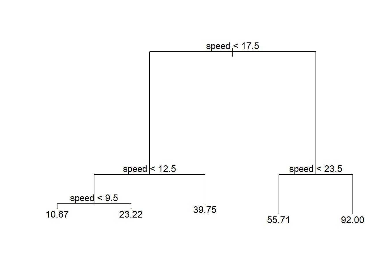
We’ve looked to two very common models:

• Multiple Linear Regression: Commonly used model with a numeric response
• Logistic Regression: Commonly used model with a binary response

These models are great ways to try and understand relationships between variables. One thing that can be a drawback (or benefit, depending) when using these models is that they are highly structured. Recall, in the MLR case we are essentially fitting some high dimensional plane to our data. If our data doesn’t follow this type of structure, the models fit can do a poor job predicting in some cases.

Instead of these structured models, we can use models that are more flexible. Let’s talk about one such type of model, the regression/classification tree!

Tree Based Methods

Tree based methods are very flexible. They attempt to split up predictor space into regions. On each region, a different prediction can then be made. Adjacent regions need not have predictions close to each other!

Recall that we have two separate tasks we could do in a supervised learning situation, regression or classification. Depending on the situation, we can create a regression or classification tree!

• Classification tree if the goal is to classify (predict) group membership

  • Usually use most prevalent class in region as the prediction

• Regression tree if the goal is to predict a continuous response

  • Usually use mean of observations in region as the prediction

These models are very easy for people to interpret! For instance, consider the tree below relating a predictor (speed) to stopping distance (dist).

library(tree) #rpart is also often used

Warning: package 'tree' was built under R version 4.1.3

fitTree <- tree(dist ~ speed, data = cars) #default splitting is deviance
plot(fitTree)
text(fitTree)

We can compare this to the simple linear regression fit to see the increased flexibility of a regression tree model.

library(tidyverse)
ggplot(cars, aes(x = speed, y = dist)) + 
  geom_point() +
  geom_smooth(method = "lm", se = FALSE, size = 2) + 
  geom_segment(x = 0, xend = 9.5, y = 10.67, yend = 10.67, col = "Orange", size = 2) +
  geom_segment(x = 9.5, xend = 12.5, y = 23.22, yend = 23.22, col = "Orange", size = 2) +
  geom_segment(x = 12.5, xend = 17.5, y = 39.75, yend = 39.75, col = "Orange", size = 2) +
  geom_segment(x = 17.5, xend = 23.5, y = 55.71, yend = 55.71, col = "Orange", size = 2) +
  geom_segment(x = 23.5, xend = max(cars$speed), y = 92, yend = 92, col = "Orange", size = 2)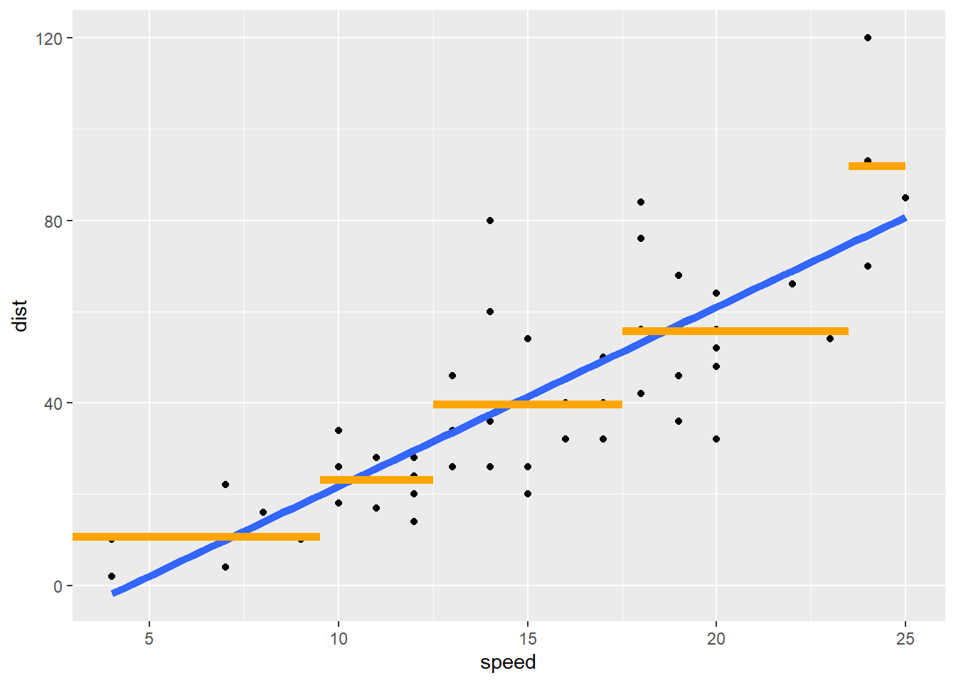

How Is a Regression Tree Fit?

Recall: Once we’ve chosen our model form, we need to fit the model to data. Generally, we can write the fitting process as the minimization of some loss function over the training data. How do we pick our splits of the predictor space in this case?

• Fit using recursive binary splitting - a greedy algorithm

• For every possible value of each predictor, we find the squared error loss based on splitting our data around that point. We then try to minimize that

  • Consider having one variable $x$. For a given observed value, call it $s$, we can think of having two regions (recall $|$ is read as ‘given’): $$R_1(s) = \{x|x < s\}\mbox{ and }R_2(s) = \{x|x \geq s\}$$
  • We seek the value of $s$ that minimize the equation $$\sum_{\mbox{all }x\mbox{ in }R_1(s)}(y_i-\bar{y}_{R_1})^2+\sum_{\mbox{all }x\mbox{ in }R_2(s)}(y_i-\bar{y}_{R_2})^2$$
  • Written more mathematically, we could say we want minimize $$min_{s} \sum_{i:x_i\in R_1(s)}(y_i-\bar{y}_{R_1})^2+\sum_{i:x_i\in R_2(s)}(y_i-\bar{y}_{R_2})^2$$

Let’s visualize this idea! Consider that basic cars data set that has a response of dist (stopping distance) and a predictor of speed. Let’s find the value of the loss functions for different splits of our speed variable.

ggplot(cars, aes(x = speed, y = dist)) + 
  geom_point()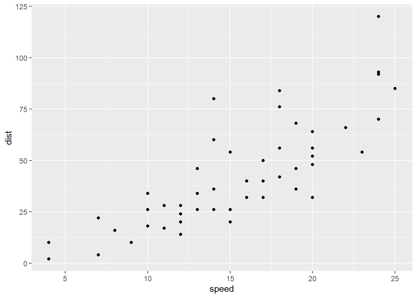

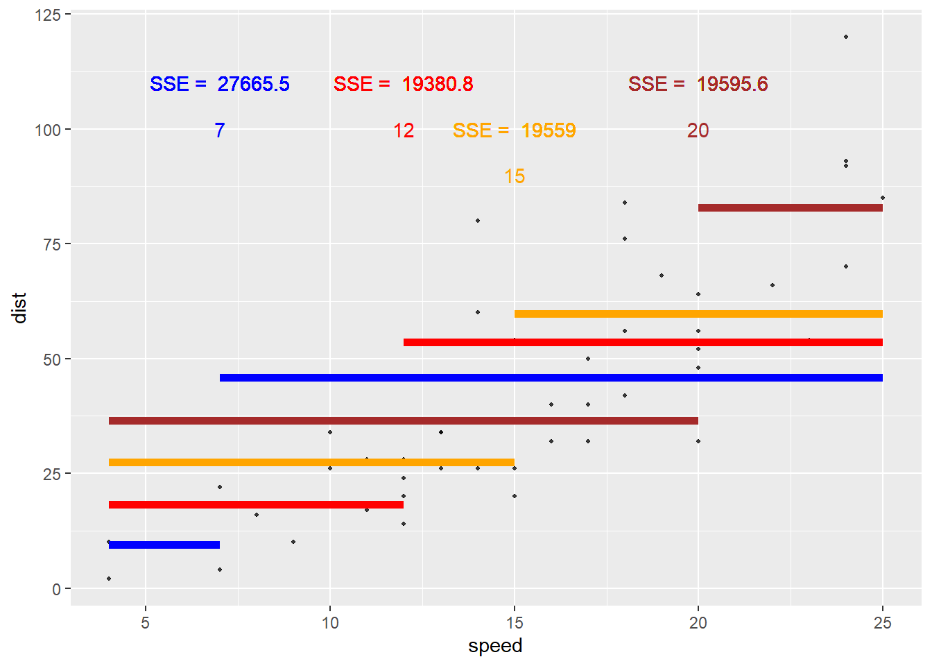
Let’s first try a split at speed = 7. The sum of squared errors based on this split is 2.766546^{4}.

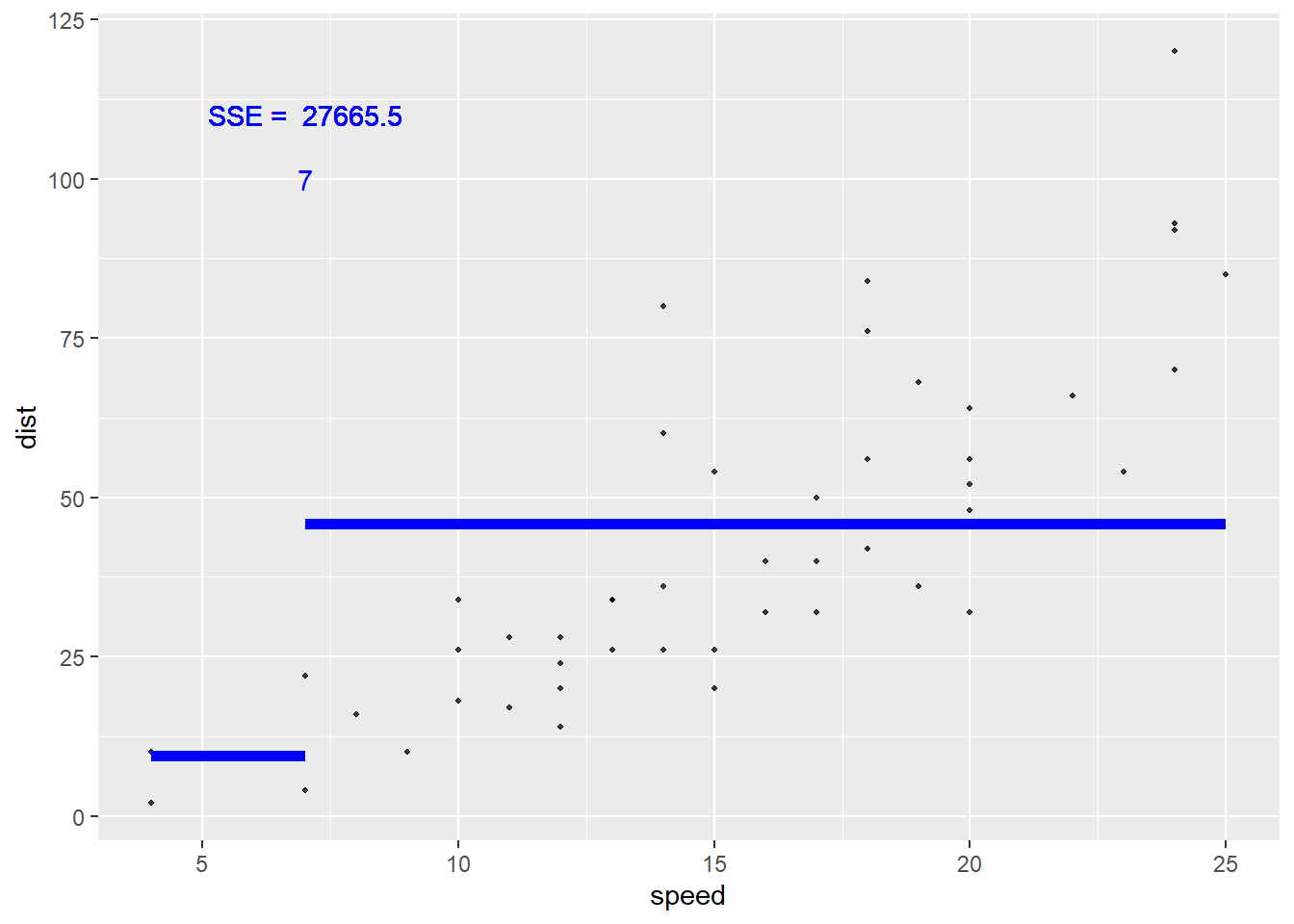
Again, this is found by taking all the points in the first region, finding the residual (from the mean, represented by the blue line here), squaring those, and summing the values. Then we repeat for the 2nd region. The sum of those two values is then the sum of squared errors (SSE) if we were to use this split.

Is that the smallest it could be? Likely not! Let’s try some other splits and see what SSE they give.

• We would try this for all possible splits (across each predictor) and choose the split that minimizes the sum of squared errors as our first split. It turns out that speed = 17.5 is the optimal splitting point for this data set.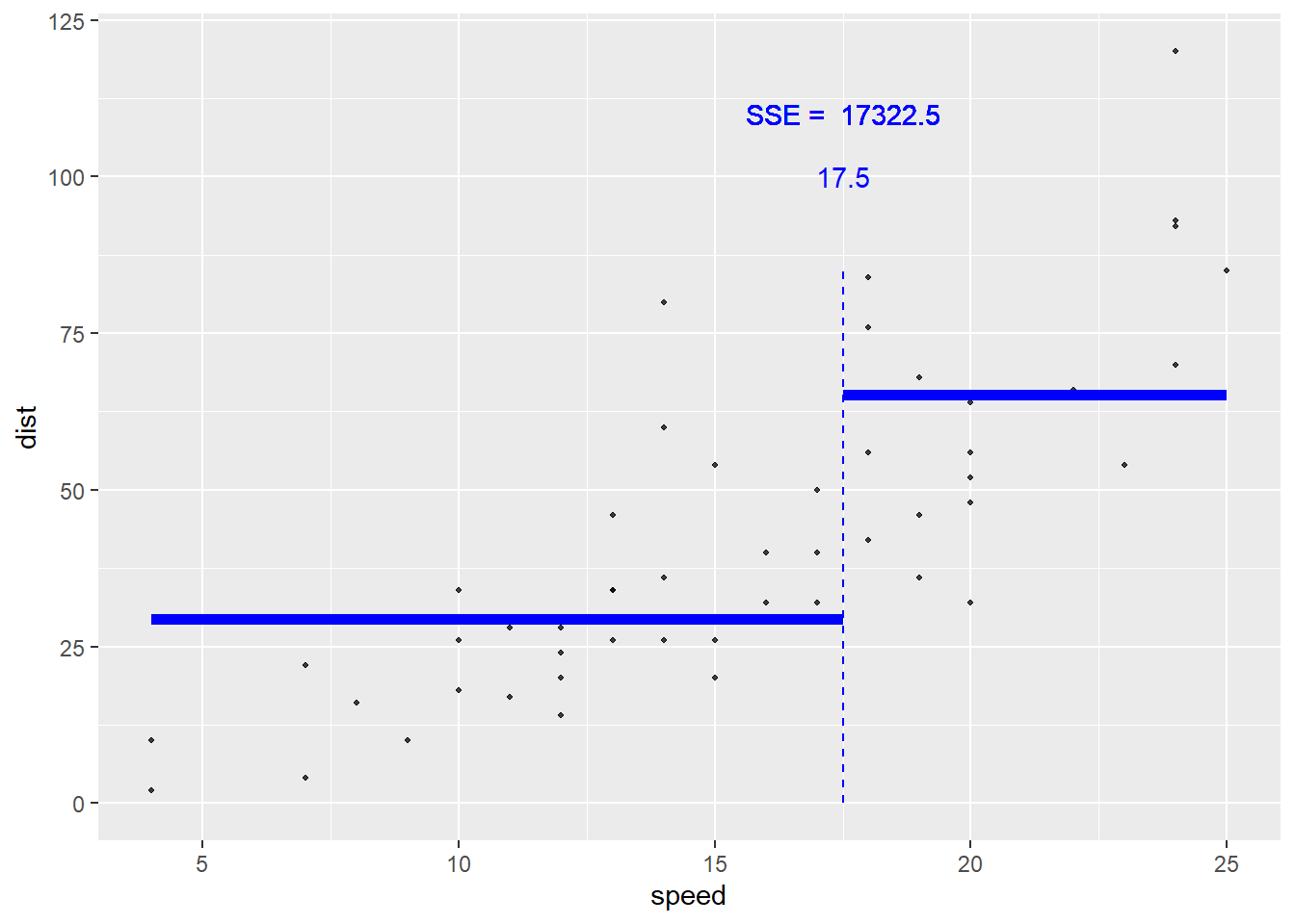

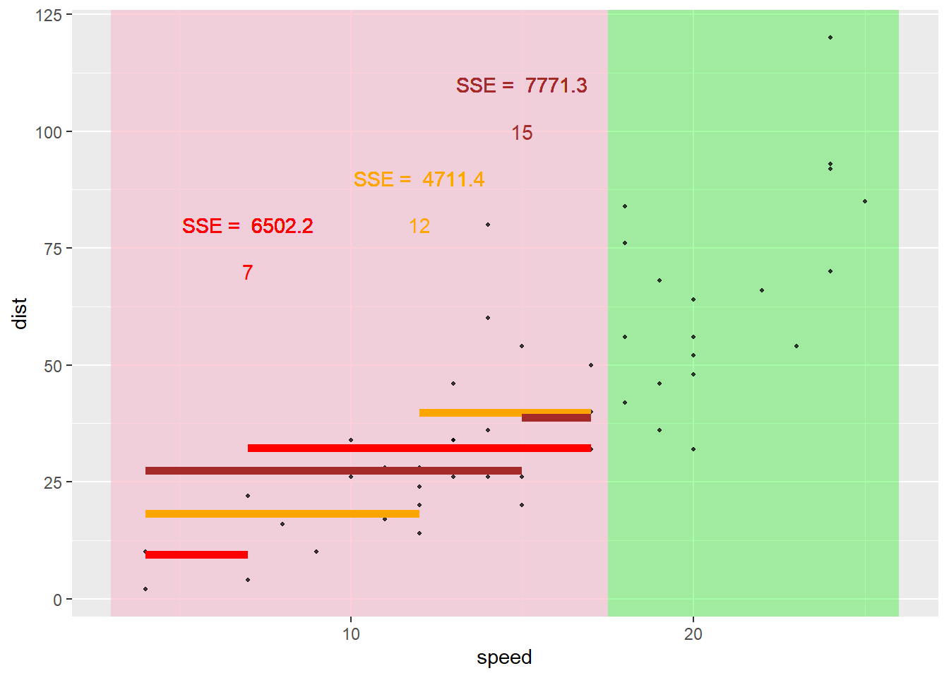
• Next, we’d go down the first branch of that split to that ‘node’. This node has all the observations corresponding to that branch. Now we repeat this process there!

• Here the best split on the lower portion is 12.5.

• Likewise, we go down the second branch to the other node and repeat the process.

• Generally, we grow a `large’ tree (many nodes)

• Trees can then be pruned back so as to not overfit the data (pruned back using some criterion like cost-complexity pruning)

• Generally, we can choose number of nodes/splits using the training/test set or cross-validation!

Fitting Regression Trees with tidymodels

• Recall the Bike data and log_selling_price as our response

set.seed(10)
library(tidyverse)
library(tidymodels)
bike_data <- read_csv("https://www4.stat.ncsu.edu/~online/datasets/bikeDetails.csv") |>
  mutate(log_selling_price = log(selling_price)) |>
  select(-selling_price)
#save creation of new variables for now!
bike_split <- initial_split(bike_data, prop = 0.7)
bike_train <- training(bike_split)
bike_test <- testing(bike_split)
bike_train

# A tibble: 742 x 7
   name     year seller_type owner km_driven ex_showroom_price log_selling_price
   <chr>   <dbl> <chr>       <chr>     <dbl>             <dbl>             <dbl>
 1 Bajaj ~  2012 Individual  1st ~     50000             54299             10.3 
 2 Honda ~  2015 Individual  1st ~      7672             54605             10.6 
 3 Bajaj ~  2005 Individual  1st ~     21885                NA              9.80
 4 Hero H~  2017 Individual  1st ~     27000                NA             10.5 
 5 Royal ~  2013 Individual  1st ~     49000                NA             11.4 
 6 Bajaj ~  2008 Individual  1st ~     19500                NA             10.3 
 7 Hero C~  2014 Individual  1st ~     38000                NA             10.5 
 8 Bajaj ~  2009 Individual  1st ~     16000                NA              9.90
 9 Hero H~  2008 Individual  3rd ~     65000                NA             10.1 
10 Bajaj ~  2019 Individual  1st ~      7600                NA             12.2 
# i 732 more rows

bike_CV_folds <- vfold_cv(bike_train, 10)

We can fit a regression tree model in a very similar way to how we fit our MLR models!

Create our Recipe for Data Preprocessing

First, let’s create our recipe.

tree_rec <- recipe(log_selling_price ~ ., data = bike_train) |>
  update_role(name, new_role = "ID") |>
  step_log(km_driven) |>
  step_rm(ex_showroom_price) |>
  step_dummy(owner, seller_type) |>
  step_normalize(all_numeric(), -all_outcomes())
tree_rec

-- Recipe ----------------------------------------------------------------------

-- Inputs 

Number of variables by role

outcome:   1
predictor: 5
ID:        1

-- Operations 

* Log transformation on: km_driven

* Variables removed: ex_showroom_price

* Dummy variables from: owner and seller_type

* Centering and scaling for: all_numeric() and -all_outcomes()

Note: We don’t need to include interaction terms in our tree based models! An interaction would imply that the effect of, say, log_km_driven depends on the year the bike was manufactured (and vice-versa). The tree structure inherently includes this type of relationship! For instance, suppose we first split on log_km_driven > 10. On the branch where log_km_driven > 10 we then split on year < 1990. Suppose those are our only two splits. We can see that the effect of year is different depending on our log_km_driven! For one side of the log_km_driven split we don’t include year at all (hence it doesn’t have an effect when considering those values of log_km_driven) and on the other side of that split we change our prediction based on year. This is exactly the idea of an interaction!

Define our Model and Engine

Next, let’s define our model. The info page here can be used to determine the right function to call and the possible engines to use for the fit.

In this case, decision_tree() with rpart as the engine will do the trick. If we click on the link for this model we can see that there are three tuning parameters we can consider:

• tree_depth: Tree Depth (type: integer, default: 30L)
• min_n: Minimal Node Size (type: integer, default: 2L)
• cost_complexity: Cost-Complexity Parameter (type: double, default: 0.01)

If we want to use CV to choose one of these, we can set its value to tune() when creating the model. Let’s use tree_depth and cost_complexity as our tuning parameters and set our min_n to 20.

In the case of decision_tree() we also need to tell tidymodels whether we are doing a regression task vs a classification task. This is done via set_mode().

tree_mod <- decision_tree(tree_depth = tune(),
                          min_n = 20,
                          cost_complexity = tune()) |>
  set_engine("rpart") |>
  set_mode("regression")

Create our Workflow

Now we use workflow() to create an object to use in our fitting processes.

tree_wkf <- workflow() |>
  add_recipe(tree_rec) |>
  add_model(tree_mod)

Use CV to Select our Tuning Parameters

Now we can use tune_grid() on our bike_CV_folds object. We just need to create a tuning grid to fit our models with. If we don’t specify one, the dials package tries to figure it out for us:

temp <- tree_wkf |> 
  tune_grid(resamples = bike_CV_folds)
temp |> 
  collect_metrics()

# A tibble: 20 x 8
   cost_complexity tree_depth .metric .estimator  mean     n std_err .config    
             <dbl>      <int> <chr>   <chr>      <dbl> <int>   <dbl> <chr>      
 1        7.50e- 6         12 rmse    standard   0.510    10  0.0175 Preprocess~
 2        7.50e- 6         12 rsq     standard   0.467    10  0.0207 Preprocess~
 3        2.80e- 8          8 rmse    standard   0.509    10  0.0174 Preprocess~
 4        2.80e- 8          8 rsq     standard   0.468    10  0.0205 Preprocess~
 5        1.66e- 3         15 rmse    standard   0.501    10  0.0158 Preprocess~
 6        1.66e- 3         15 rsq     standard   0.479    10  0.0182 Preprocess~
 7        5.79e-10          2 rmse    standard   0.538    10  0.0196 Preprocess~
 8        5.79e-10          2 rsq     standard   0.396    10  0.0209 Preprocess~
 9        4.05e- 9          3 rmse    standard   0.510    10  0.0181 Preprocess~
10        4.05e- 9          3 rsq     standard   0.456    10  0.0193 Preprocess~
11        1.24e- 3          6 rmse    standard   0.503    10  0.0158 Preprocess~
12        1.24e- 3          6 rsq     standard   0.477    10  0.0193 Preprocess~
13        5.68e- 2          5 rmse    standard   0.543    10  0.0202 Preprocess~
14        5.68e- 2          5 rsq     standard   0.382    10  0.0165 Preprocess~
15        1.82e- 6         12 rmse    standard   0.510    10  0.0175 Preprocess~
16        1.82e- 6         12 rsq     standard   0.467    10  0.0207 Preprocess~
17        5.23e- 8          9 rmse    standard   0.509    10  0.0175 Preprocess~
18        5.23e- 8          9 rsq     standard   0.468    10  0.0208 Preprocess~
19        5.47e- 5          9 rmse    standard   0.509    10  0.0175 Preprocess~
20        5.47e- 5          9 rsq     standard   0.468    10  0.0208 Preprocess~

We can see that the cost_complexity parameter and tree_depth parameters are randomly varied and results are returned.

If we want to set the number of the values ourselves, we can use grid_regular() instead. By specifying a vector or levels we can say how many of each tuning parameter we want. grid_regular() then finds all combinations of the values of each (here 10*5 = 50 combinations).

tree_grid <- grid_regular(cost_complexity(),
                          tree_depth(),
                          levels = c(10, 5))

Now we use tune_grid() with this grid specified.

tree_fits <- tree_wkf |> 
  tune_grid(resamples = bike_CV_folds,
            grid = tree_grid)
tree_fits

# Tuning results
# 10-fold cross-validation 
# A tibble: 10 x 4
   splits           id     .metrics           .notes          
   <list>           <chr>  <list>             <list>          
 1 <split [667/75]> Fold01 <tibble [100 x 6]> <tibble [0 x 3]>
 2 <split [667/75]> Fold02 <tibble [100 x 6]> <tibble [0 x 3]>
 3 <split [668/74]> Fold03 <tibble [100 x 6]> <tibble [0 x 3]>
 4 <split [668/74]> Fold04 <tibble [100 x 6]> <tibble [0 x 3]>
 5 <split [668/74]> Fold05 <tibble [100 x 6]> <tibble [0 x 3]>
 6 <split [668/74]> Fold06 <tibble [100 x 6]> <tibble [0 x 3]>
 7 <split [668/74]> Fold07 <tibble [100 x 6]> <tibble [0 x 3]>
 8 <split [668/74]> Fold08 <tibble [100 x 6]> <tibble [0 x 3]>
 9 <split [668/74]> Fold09 <tibble [100 x 6]> <tibble [0 x 3]>
10 <split [668/74]> Fold10 <tibble [100 x 6]> <tibble [0 x 3]>

Looking at the tree_fits object isn’t super useful. It has all the info but we need to pull it out. As we see above, we can use collect_metrics() to combine the metrics across the folds.

tree_fits |>
  collect_metrics()

# A tibble: 100 x 8
   cost_complexity tree_depth .metric .estimator  mean     n std_err .config    
             <dbl>      <int> <chr>   <chr>      <dbl> <int>   <dbl> <chr>      
 1    0.0000000001          1 rmse    standard   0.561    10  0.0190 Preprocess~
 2    0.0000000001          1 rsq     standard   0.338    10  0.0176 Preprocess~
 3    0.000000001           1 rmse    standard   0.561    10  0.0190 Preprocess~
 4    0.000000001           1 rsq     standard   0.338    10  0.0176 Preprocess~
 5    0.00000001            1 rmse    standard   0.561    10  0.0190 Preprocess~
 6    0.00000001            1 rsq     standard   0.338    10  0.0176 Preprocess~
 7    0.0000001             1 rmse    standard   0.561    10  0.0190 Preprocess~
 8    0.0000001             1 rsq     standard   0.338    10  0.0176 Preprocess~
 9    0.000001              1 rmse    standard   0.561    10  0.0190 Preprocess~
10    0.000001              1 rsq     standard   0.338    10  0.0176 Preprocess~
# i 90 more rows

As done in the tutorial, we can plot these to gain some insight:

tree_fits %>%
  collect_metrics() %>%
  mutate(tree_depth = factor(tree_depth)) %>%
  ggplot(aes(cost_complexity, mean, color = tree_depth)) +
  geom_line(size = 1.5, alpha = 0.6) +
  geom_point(size = 2) +
  facet_wrap(~ .metric, scales = "free", nrow = 2) +
  scale_x_log10(labels = scales::label_number()) +
  scale_color_viridis_d(option = "plasma", begin = .9, end = 0)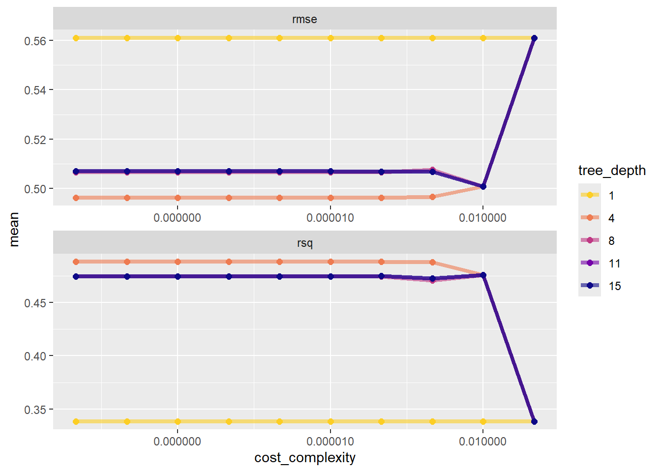

Ideally, we probably want to sort this by the smallest rmse value. Let’s also filter down to just looking at rmse.

tree_fits |>
  collect_metrics() |>
  filter(.metric == "rmse") |>
  arrange(mean)

# A tibble: 50 x 8
   cost_complexity tree_depth .metric .estimator  mean     n std_err .config    
             <dbl>      <int> <chr>   <chr>      <dbl> <int>   <dbl> <chr>      
 1    0.0000000001          4 rmse    standard   0.496    10  0.0163 Preprocess~
 2    0.000000001           4 rmse    standard   0.496    10  0.0163 Preprocess~
 3    0.00000001            4 rmse    standard   0.496    10  0.0163 Preprocess~
 4    0.0000001             4 rmse    standard   0.496    10  0.0163 Preprocess~
 5    0.000001              4 rmse    standard   0.496    10  0.0163 Preprocess~
 6    0.00001               4 rmse    standard   0.496    10  0.0163 Preprocess~
 7    0.0001                4 rmse    standard   0.496    10  0.0163 Preprocess~
 8    0.001                 4 rmse    standard   0.496    10  0.0162 Preprocess~
 9    0.01                  4 rmse    standard   0.498    10  0.0176 Preprocess~
10    0.01                  8 rmse    standard   0.498    10  0.0176 Preprocess~
# i 40 more rows

The function select_best() can be used to grab the best model’s tuning parameter values. We also should specify which metric!

tree_best_params <- select_best(tree_fits, metric = "rmse")
tree_best_params

# A tibble: 1 x 3
  cost_complexity tree_depth .config              
            <dbl>      <int> <chr>                
1    0.0000000001          4 Preprocessor1_Model11

(After this initial phase, we might also want to fit a finer grid of tuning parameter values near the current ‘best’ ones!) Now we can finalize our model on the training set by fitting this chosen model via finalize_workflow().

tree_final_wkf <- tree_wkf |>
  finalize_workflow(tree_best_params)

Now that we’ve set up how to fit the final model, let’s do it via last_fit() on the bike_split object.

tree_final_fit <- tree_final_wkf |>
  last_fit(bike_split)
tree_final_fit

# Resampling results
# Manual resampling 
# A tibble: 1 x 6
  splits            id               .metrics .notes   .predictions .workflow 
  <list>            <chr>            <list>   <list>   <list>       <list>    
1 <split [742/319]> train/test split <tibble> <tibble> <tibble>     <workflow>

This object has information about how the final fitted model (fit on the entire training data set) performs on the test set. We can see the metrics more clearly using collect_metrics().

tree_final_fit |>
  collect_metrics()

# A tibble: 2 x 4
  .metric .estimator .estimate .config             
  <chr>   <chr>          <dbl> <chr>               
1 rmse    standard       0.565 Preprocessor1_Model1
2 rsq     standard       0.445 Preprocessor1_Model1

As done in the tutorial, we could pull out this fit and learn more about it.

tree_final_model <- extract_workflow(tree_final_fit) 
tree_final_model

== Workflow [trained] ==========================================================
Preprocessor: Recipe
Model: decision_tree()

-- Preprocessor ----------------------------------------------------------------
4 Recipe Steps

* step_log()
* step_rm()
* step_dummy()
* step_normalize()

-- Model -----------------------------------------------------------------------
n= 742 

node), split, n, deviance, yval
      * denotes terminal node

 1) root 742 352.956900 10.721500  
   2) year< 0.1604381 354 118.136200 10.304490  
     4) year< -0.9711688 99  42.945090  9.955315  
       8) km_driven>=-0.07668815 80  24.027690  9.812273  
        16) year< -1.423811 52  11.224130  9.659656 *
        17) year>=-1.423811 28   9.343018 10.095710 *
       9) km_driven< -0.07668815 19  10.388380 10.557600 *
     5) year>=-0.9711688 255  58.435060 10.440050  
      10) km_driven>=-0.1109097 205  33.439120 10.355390  
        20) year< -0.518526 80  12.341380 10.225880 *
        21) year>=-0.518526 125  18.897350 10.438270 *
      11) km_driven< -0.1109097 50  17.502590 10.787150  
        22) year< -0.2922047 16   6.876996 10.503040 *
        23) year>=-0.2922047 34   8.726354 10.920850 *
   3) year>=0.1604381 388 117.094000 11.101970  
     6) year< 0.6130808 149  29.735310 10.800920  
      12) km_driven>=-0.5047722 121  20.838220 10.751970  
        24) owner_X2nd.owner>=1.178863 15   1.468796 10.451540 *
        25) owner_X2nd.owner< 1.178863 106  17.823910 10.794490 *
      13) km_driven< -0.5047722 28   7.354383 11.012450  
        26) km_driven< -1.218805 10   1.952084 10.880130 *
        27) km_driven>=-1.218805 18   5.129964 11.085950 *
     7) year>=0.6130808 239  65.435960 11.289650  
      14) km_driven>=-1.236697 179  35.914190 11.164620  
        28) km_driven>=0.1002281 52   8.612033 10.998670 *
        29) km_driven< 0.1002281 127  25.283800 11.232560 *
      15) km_driven< -1.236697 60  18.374510 11.662680  
        30) km_driven>=-2.026019 38   8.605414 11.552500 *
        31) km_driven< -2.026019 22   8.511043 11.852980 *

Plotting is definitely the better way to view this!

tree_final_model %>%
  extract_fit_engine() %>%
  rpart.plot::rpart.plot(roundint = FALSE)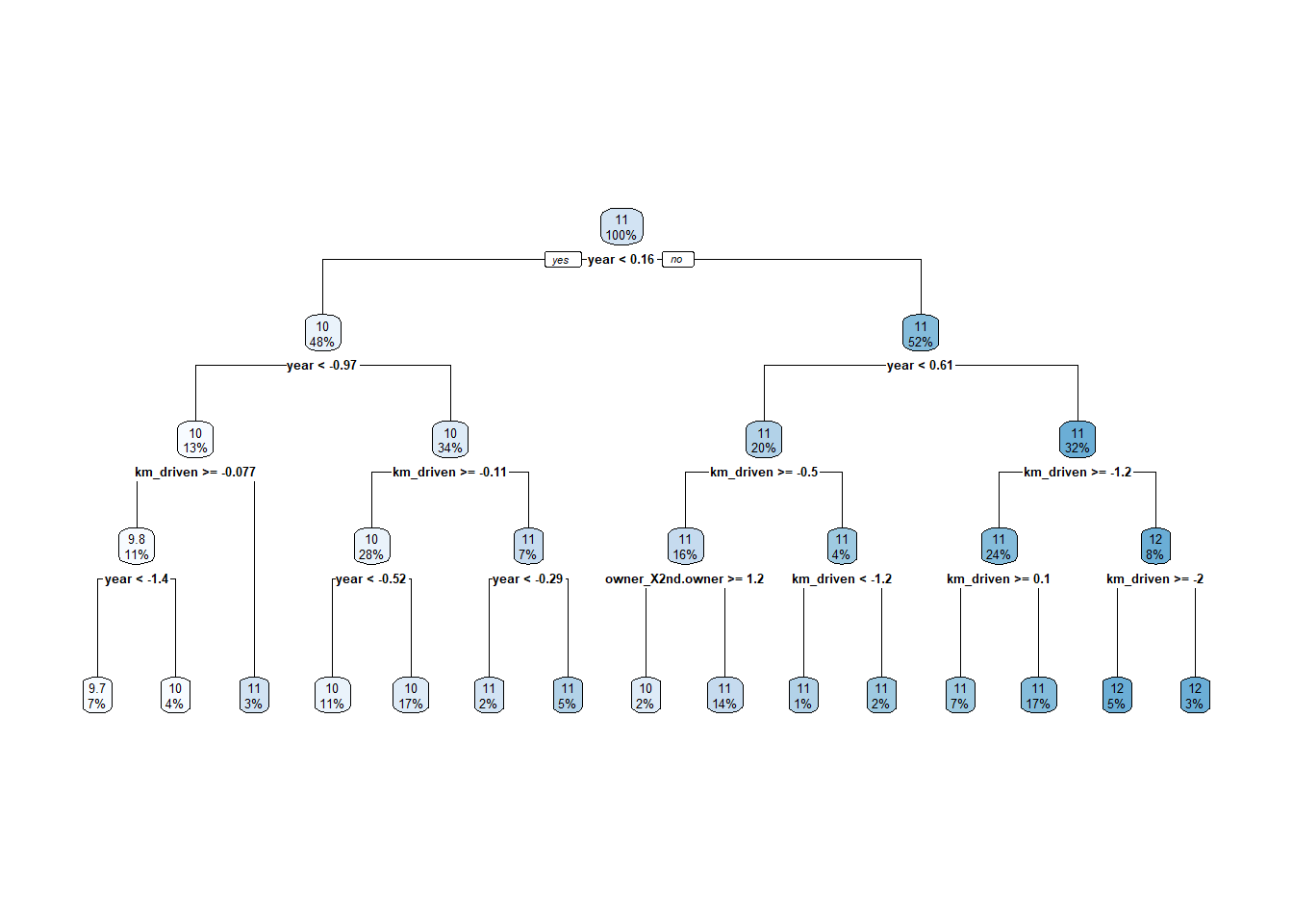

Comparing to Our LASSO and MLR Fits

Recall, we fit MLR models and LASSO models to this data set. We can pull those back up to determine which model did the best overall on the test set. Then we can get an overall ‘best’ model and fit that model to the entire data set!

Classification Trees

Classification trees are very similar to regression trees except, of course, our response is a categorical variable. This means that we don’t use the same loss functions nor metrics, but we still split the predictor space up into regions. We then can make our prediction based on which bin an observation ends up in. Most often, we use the most prevalent class in a bin as our prediction.

Recap and Pros & Cons

• Trees are a nonlinear model that can be more flexible than linear models.

Pros:

• Simple to understand and easy to interpret output
  
• Predictors don’t need to be scaled. Unlike algorithms like the LASSO, having all the predictors on different scales makes no difference in the choosing of regions.
• No statistical assumptions necessary to get the fit (although this is true for least squares regression as well)
• Built in variable selection based on the algorithm!

Cons:

• Small changes in data can vastly change tree

  • The lack of ‘sharing’ information with nearby data points makes this algorithm more variable. Given a new data set from the same situation, the splits we get for the tree can differ quite a bit! That isn’t ideal as we’d like to have stable results across data sets collected on the same population.

• No optimal algorithm for choosing splits exists.

  • We saw the use of a greedy algorithm to select our regions in the regression tree case. This is a greedy algorithm because it is only looking one step ahead to find the best split. There might be a split at this step that creates a great future split. However, we may never find it because we only ever look at the best thing we can do at the current split!

• Need to prune or use CV to determine the model.

  • With MLR models, CV isn’t used at all. However, here we really need to prune the tree and/or use CV to figure out the optimal size of the tree to build!

Use the table of contents on the left or the arrows at the bottom of this page to navigate to the next learning material!