Prediction & Training/Test Sets

In this course we focus on the predictive modeling paradigm. In the end, we’ll often fit different families of models (say some multiple linear regression models, a tree based model, and a random forest model) to a given data set. We’ll then judge those models using some model metric to determine which model is best at predicting!

Let’s break down this process into a few steps.

Predictive Modeling Idea

First we’ll choose a form for a model. The types of models to consider often depends on the subject matter at hand. In this course, we’ll cover a few general types (or families) of models.

Once we’ve chosen a model type, we fit the model using some algorithm. Usually, we can write this fitting process in terms of minimizing some loss function.

We then need to determine the quality of predictions made by the model. We use a model metric to do this. Quite often, the loss function and model metric are the same, but this isn’t always the case!

For numeric response, the most common model metric is mean squared error (MSE) or root mean squared error (RMSE). For a categorical reponse, the most commmon model metrics are accuracy and log-loss (discussed in detail later).

Training vs Test Sets

Ideally we want our model to predict well for observations it has yet to see. We want to avoid overfitting to the data we train our model on.

The evaluation of predictions over the observations used to fit or train the model is called the training (set) error

• Let $y_i$ denote an observed value and $\hat{y}_i$ denote our prediction for that observation. If RMSE was our metric:

$$\mbox{Training RMSE} = \sqrt{\frac{1}{\mbox{# of obs used to fit model}}\sum_{\mbox{obs used to fit model}}(y_i-\hat{y}_i)^2}$$

• If we only consider this error, we’ll have no idea how the model will fare on data it hasn’t seen!

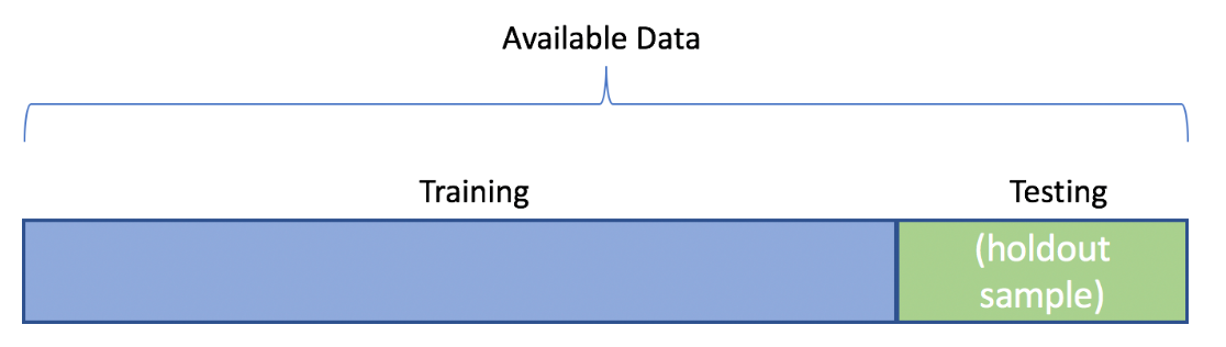
One method to obtain a better idea about model performance is to randomly split the data into a training set and test set.

• On the training set we can fit (or train) our models
• We can then predict for the test set observations and judge effectiveness with our metric

Example of Fitting and Evaluating Models

Consider our data set on motorcycle sale prices

library(tidyverse)
bike_data <- read_csv("https://www4.stat.ncsu.edu/~online/datasets/bikeDetails.csv")
bike_data <- bike_data |> 
  mutate(log_selling_price = log(selling_price), 
         log_km_driven = log(km_driven)) |>
  select(log_km_driven, log_selling_price, everything())
bike_data

# A tibble: 1,061 x 9
   log_km_driven log_selling_price name    selling_price  year seller_type owner
           <dbl>             <dbl> <chr>           <dbl> <dbl> <chr>       <chr>
 1          5.86             12.1  Royal ~        175000  2019 Individual  1st ~
 2          8.64             10.7  Honda ~         45000  2017 Individual  1st ~
 3          9.39             11.9  Royal ~        150000  2018 Individual  1st ~
 4         10.0              11.1  Yamaha~         65000  2015 Individual  1st ~
 5          9.95              9.90 Yamaha~         20000  2011 Individual  2nd ~
 6         11.0               9.80 Honda ~         18000  2010 Individual  1st ~
 7          9.74             11.3  Honda ~         78500  2018 Individual  1st ~
 8         10.6              12.1  Royal ~        180000  2008 Individual  2nd ~
 9         10.4              10.3  Hero H~         30000  2010 Individual  1st ~
10         10.6              10.8  Bajaj ~         50000  2016 Individual  1st ~
# i 1,051 more rows
# i 2 more variables: km_driven <dbl>, ex_showroom_price <dbl>

Here our response variable is the log_selling_price = ln(selling_price). We could consider the family of multiple linear regression (MLR) models with differing predictors (x variables).

• The basic MLR model with $p$ predictors models the average response variable given the predictors (that’s what $E(Y|x_1,x_2,...,x_p)$ represents, the average or expected $Y$, given (that’s what the vertical bar means) the values of $x_1$, $x_2$, …, $x_p$) as a linear function (linear in the parameter terms).

$$E(Y|x_1, x_2, ..., x_p) = \beta_0+\beta_1x_1+\beta_2x_2+...+\beta_px_p$$

• $\beta_0$ is the intercept and each $\beta_j$ is a slope term associated with a predictor variable.
• As with SLR, we could model the error term with a Normal distribution if we were interested in making inference on the parameters

These basic models find coefficients that minimize the sum of squared residuals (i.e. uses squared error loss to fit the model).

• MLR modeling fitting criterion (the ‘hats’ just imply the parameters are estimates rather than the ‘true’ underlying values):

$$min_{\hat{\beta}'s}\sum_{i=1}^{n}(y_i-(\hat{\beta}_0+\hat{\beta}_1x_{1i}+...+\hat{\beta}_px_{pi}))^2$$

This turns out to be equivalent to doing maximum likelihood estimation with the iid error Normal, constant variance, assumption!

• Consider three competing MLR models:

  • $\mbox{Model 1: log_selling_price = intercept + slope*year + Error}$
  • $\mbox{Model 2: log_selling_price = intercept + slope*log_km_driven + Error}$
  • $\mbox{Model 3: log_selling_price = intercept + slope*log_km_driven + slope*year + Error}$

We can split the data randomly into a training set and a testing set. There are a lot of ways to do this. We’ll use the rsample::initial_split() function.

• We commonly use an 80/20 or 70/30 training/test split. The proportion used in this split really depends on the amount of data you have and your subject matter expertise. More data in the test set means a better estimate of the model’s performance. However, less data in the training set means a more variable model (bigger changes in predictions from data set to data set).

• Let’s split our bike_data into a training and test set.

  • Use initial_split() to create an initial object
  • Use training() and testing() on that object to create the two data sets (note the number of observations in each set below!)

library(tidymodels)
set.seed(10)
bike_split <- initial_split(bike_data, prop = 0.7)
bike_train <- training(bike_split)
bike_test <- testing(bike_split)
bike_train

# A tibble: 742 x 9
   log_km_driven log_selling_price name    selling_price  year seller_type owner
           <dbl>             <dbl> <chr>           <dbl> <dbl> <chr>       <chr>
 1         10.8              10.3  Bajaj ~         30000  2012 Individual  1st ~
 2          8.95             10.6  Honda ~         40000  2015 Individual  1st ~
 3          9.99              9.80 Bajaj ~         18000  2005 Individual  1st ~
 4         10.2              10.5  Hero H~         35000  2017 Individual  1st ~
 5         10.8              11.4  Royal ~         85000  2013 Individual  1st ~
 6          9.88             10.3  Bajaj ~         30000  2008 Individual  1st ~
 7         10.5              10.5  Hero C~         35000  2014 Individual  1st ~
 8          9.68              9.90 Bajaj ~         20000  2009 Individual  1st ~
 9         11.1              10.1  Hero H~         25000  2008 Individual  3rd ~
10          8.94             12.2  Bajaj ~        200000  2019 Individual  1st ~
# i 732 more rows
# i 2 more variables: km_driven <dbl>, ex_showroom_price <dbl>

bike_test

# A tibble: 319 x 9
   log_km_driven log_selling_price name    selling_price  year seller_type owner
           <dbl>             <dbl> <chr>           <dbl> <dbl> <chr>       <chr>
 1          8.64             10.7  Honda ~         45000  2017 Individual  1st ~
 2          9.39             11.9  Royal ~        150000  2018 Individual  1st ~
 3          7.03             12.8  Yamaha~        365000  2019 Individual  1st ~
 4          7.44             12.1  Jawa 42        185000  2020 Individual  1st ~
 5         10.9              10.1  Suzuki~         25000  2012 Individual  1st ~
 6         11.0               9.62 Hero P~         15000  2008 Individual  1st ~
 7          7.60             12.1  Jawa S~        180000  2019 Individual  1st ~
 8         10.1              10.6  Honda ~         42000  2017 Individual  1st ~
 9          9.21              9.95 Hero H~         21000  2009 Individual  1st ~
10          9.95             10.7  Hero G~         45000  2018 Individual  1st ~
# i 309 more rows
# i 2 more variables: km_driven <dbl>, ex_showroom_price <dbl>

We can fit or train these models on the training set. Recall we use lm() to easily fit an MLR model via formula notation. With formula notation we put our response variable on the left and our model for the predictors on the right. The model can include interactions, non-linear terms, etc. If we just want ‘main effects’ we separate predictors with + on the right hand side (we’ll cover this in more detail later!)

• Let’s fit our three models and save them as objects.

reg1 <- lm(log_selling_price ~ year, data = bike_train)
coef(reg1)

  (Intercept)          year 
-186.17235057    0.09777273 

reg2 <- lm(log_selling_price ~ log_km_driven, data = bike_train)
coef(reg2)

  (Intercept) log_km_driven 
   14.6228627    -0.3899342 

reg3 <- lm(log_selling_price ~ year + log_km_driven, data = bike_train)
coef(reg3)

  (Intercept)          year log_km_driven 
-131.66741960    0.07191291   -0.24274055 

Now we have the fitted models. Want to use them to predict the response

• $\mbox{Model 1: } \widehat{\mbox{log_selling_price}} = -186.1724 + 0.0978*\mbox{year}$
• $\mbox{Model 2: } \widehat{\mbox{log_selling_price}} = 14.6229 -0.3899*\mbox{log_km_driven}$
• $\mbox{Model 3: } \widehat{\mbox{log_selling_price}} = -131.6674 + 0.0719*\mbox{year}-0.2427*\mbox{log_km_driven}$

To get predictions from our model, we use the predict() function and specify the newdata we want to predict for as a data frame with column names matching our predictors in our models. If we don’t specify any newdata, it returns the predictions made on the training data.

• We can see the first few predictions on the training data from the first model via the code below

#year values the predictions are for
bike_train$year |> head()

[1] 2012 2015 2005 2017 2013 2008

#predictions made with our first model
predict(reg1) |> head()

        1         2         3         4         5         6 
10.546377 10.839696  9.861968 11.035241 10.644150 10.155287 

Let’s use RMSE as our metric. Although not how we want to compare our models, we can obtain the training RMSE easily with predict(). Let’s code it up ourselves and also yardstick::rmse_vec() to find it (this is the tidymodels way).

#our own calculation for training RMSE
sqrt(mean((bike_train$log_selling_price - predict(reg1))^2))

[1] 0.5378694

• Now we can supply the actual responses and the model predictions to yardstick::rmse_vec()

#using yardstick
yardstick::rmse_vec(bike_train$log_selling_price, predict(reg1))

[1] 0.5378694

#second and third models
#using yardstick
rmse_vec(bike_train$log_selling_price, predict(reg2))

[1] 0.5669127

#using yardstick
rmse_vec(bike_train$log_selling_price, predict(reg3))

[1] 0.4924924

• These values represent a measure of quality of prediction by these models (as judged by our metric RMSE).

• This estimate of RMSE for the predictions is too optimistic compared to how the model would perform with new data!

• Really, what we want to compare is how the models do on data they weren’t trained on.

• We want to find this type of metric on the test set. That means we want to use the truth from the test set ($y_i$ for the test set) and compare that to predictions made for that test set observation ($\hat{y}_i$).

$$\mbox{Test Set RMSE} = \sqrt{\frac{1}{n_{test}}\sum_{i=1}^{n_{test}}(y_i-\hat{y}_i)^2}$$

To do this in R we need to tell predict() about the newdata being the test set (bike_test). As this is a data frame with columns for our predictors, we can just pass the entire data frame for ease and predict() uses appropriate/needed columns to find our predictions.

#look at a few observations and predictions
bike_test |>
  select(log_km_driven, log_selling_price) |>
  mutate(model_1_preds = predict(reg1, newdata = bike_test))

# A tibble: 319 x 3
   log_km_driven log_selling_price model_1_preds
           <dbl>             <dbl>         <dbl>
 1          8.64             10.7           11.0
 2          9.39             11.9           11.1
 3          7.03             12.8           11.2
 4          7.44             12.1           11.3
 5         10.9              10.1           10.5
 6         11.0               9.62          10.2
 7          7.60             12.1           11.2
 8         10.1              10.6           11.0
 9          9.21              9.95          10.3
10          9.95             10.7           11.1
# i 309 more rows

• Now let’s find the test set error for each model

#obtain the test set RMSE for each model
rmse_vec(bike_test$log_selling_price, predict(reg1, newdata = bike_test))

[1] 0.5746992

rmse_vec(bike_test$log_selling_price, predict(reg2, newdata = bike_test))

[1] 0.6548019

rmse_vec(bike_test$log_selling_price, predict(reg3, newdata = bike_test))

[1] 0.554596

We see that our third model with both year and log_km_driven gives a better (by our metric) set of predictions!

When choosing a model, if the RMSE values were ‘close’, we’d want to consider the interpretability of the model (and perhaps the assumptions required by each model if we wanted to do inference too!)

• Note: we can do this with yardstick::rmse() if our predictions are in the data frame. rmse() takes in the data as the first argument, the truth column as the second, and the estimate (or predictions) as the third.

#look at a few observations and predictions
bike_test |>
  select(log_selling_price, log_km_driven) |>
  mutate(model_1_preds = predict(reg1, newdata = bike_test)) |>
  rmse(truth = log_selling_price, estimate = model_1_preds)

# A tibble: 1 x 3
  .metric .estimator .estimate
  <chr>   <chr>          <dbl>
1 rmse    standard       0.575

Recap

We generally need to go through a few steps when training and testing our model(s):

• Choose form of model
• Fit model to data using some algorithm
  • Usually can be written as a problem where we minimize some loss function
• Evaluate the model using a metric
  • RMSE very common for a numeric response
• Ideally we want our model to predict well for observations it has yet to see!

Use the table of contents on the left or the arrows at the bottom of this page to navigate to the next learning material!