Databases and Basic SQL

Published

2025-05-09

We’ve seen the use of flat files to store data (delimited data files). These files often have a file extension of .csv, .txt, or .dat.

However, we often have multiple data sources around one problem. For instance, our Lahman package we’ve been using has information about Major League Baseball players’ batting, pitching, and personal information.

There are many data tables (essentially each could be a data frame). Below is information about the structure of these data tables and how they relate.

When we have multiple data sets (or sources) a database is often used along with a database management system (DBMS)
The data, the DBMS, and the applications associated with them are often simply called a database

Database - Organized Collection of Data

For most standard databases, we usually think of a bunch of 2D tables that are related by keys. We might refer to this as a relational database.

Consider the Lahman diagram:

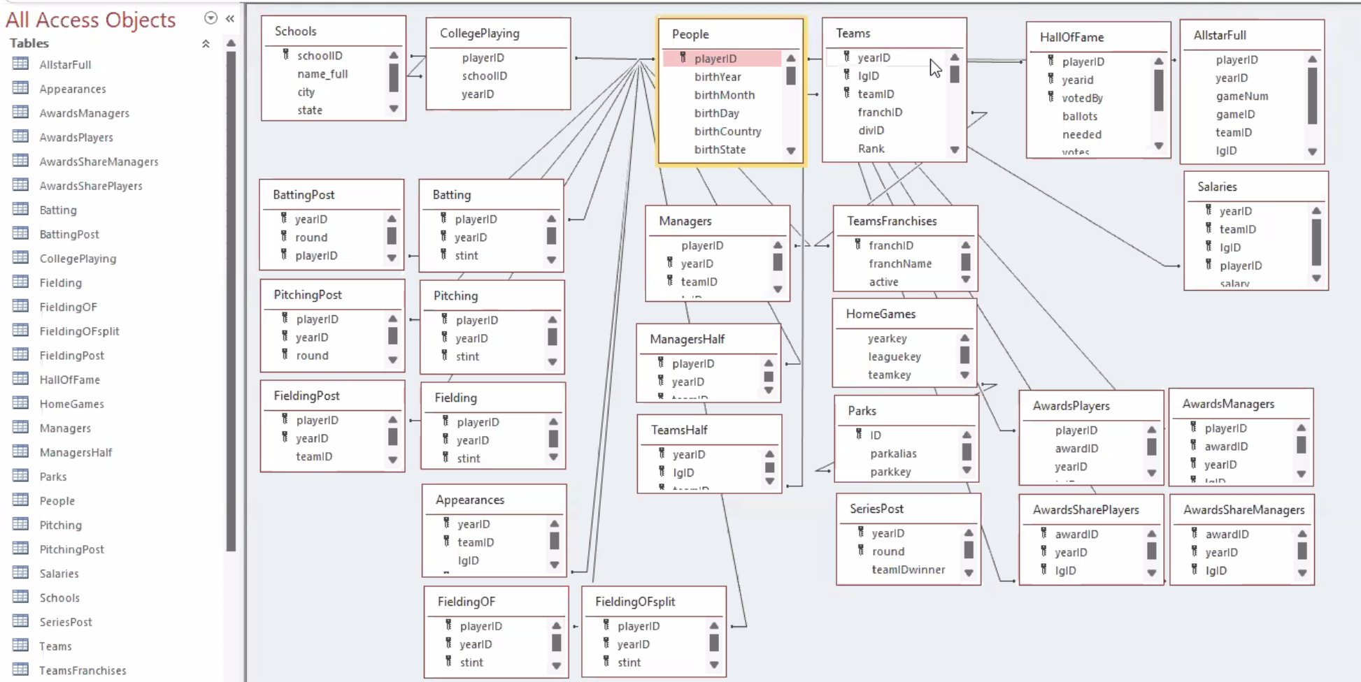
Each rectangle represents one data table. We can see that the playerID variable is common across many of these tables. This is a variable that relates the tables to each other. A common task is then to combine separate data tables in order to do an analysis.

Currently, the Lahman data sets are not in a data base. They are simply stored in our package. We can put them into a database for some practice!

Databases Systems

There are many common types of relational databases management systems (RDBMS). Some of the more popular database types are:

Most of these RDBMS have their own Structured Query Language (SQL) that provides a language for getting information from tables in the database. The SQL languages have the same core functionality and syntax that is vital to learn as a data scientist!

Actions on Databases

There are a few common actions we often want to perform on a database (CRUD actions):

Create data (add rows or a table to the database)
Read data (return data from a table in the database)
Update data
Delete data
Plus: Provide access control, monitoring, tuning, and backup/recovery

The SQL code allows us to do these operations. Luckily, the logic for doing the querying is shared with the actions we do in dplyr! We’ll be able to query databases using dplyr commands and compare that to the equivalent SQL commands. The big idea is to get the logic down. Once you have that, it is just learning the syntax.

Databases in R: Connecting

The first step in dealing with a database is to connect yourR session to it so you can do your CRUD actions. To connect we use the DBI package. The dbConnect() function allows us to connect to a database. Here is some generic code for using that function:

library(DBI)
con <- dbConnect(data_base_type_goes_here_usually_requires_a_package, 
  host = "hostname.website",
  user = "username",
  password = rstudioapi::askForPassword("DB password")
)

This code tellsR where the connection exists (host) and, if you need to login to gain access, the way in which you could specify your username and password.

The first argument specifies the type of database you are connecting to. Most commonly you’ll need to download an appropriate package and put something like the following:

RSQLite::SQLite() for RSQLite
RMySQL::MySQL() for RMySQL
RPostgreSQL::PostgreSQL() for RPostgreSQL
odbc::odbc() for Open Database Connectivity
bigrquery::bigquery() for google’s bigQuery

Databases in R: Querying a Table

Once connect, you can use tbl() to reference a table in the database. Notice our first argument is the connection we made above.

new_data <- tbl(con, "name_of_table")

We can then use SQL code or dplyr code (which actually calls code from a package called dbplyr) to query things.

Databases in R: Ending Your Connection

When done working, it is good practice to disconnect from the database via the dbDisconnect() function.

dbDisconnect(con)

Databases Example

A Lahman RSQLite exists at https://www4.stat.ncsu.edu/~online/datasets/lahman.db. We’ll do some practice with this! Make sure you install the RSQLite package if you don’t have that already.

You’ll need to download the .db file and place it in a place you know (perhaps your project directory or the directory your .qmd file lives in.)

Then you can run this code to connect to the database!

library(DBI)
con <- dbConnect(RSQLite::SQLite(), "data/lahman.db")

First, let’s list out the tables with DBI::dbListTables()

dbListTables(con)

 [1] "AllstarFull"         "Appearances"         "AwardsManagers"     
 [4] "AwardsPlayers"       "AwardsShareManagers" "AwardsSharePlayers" 
 [7] "Batting"             "BattingPost"         "CollegePlaying"     
[10] "Fielding"            "FieldingOF"          "FieldingOFsplit"    
[13] "FieldingPost"        "HallOfFame"          "HomeGames"          
[16] "LahmanData"          "Managers"            "ManagersHalf"       
[19] "Parks"               "People"              "Pitching"           
[22] "PitchingPost"        "Salaries"            "Schools"            
[25] "SeriesPost"          "Teams"               "TeamsFranchises"    
[28] "TeamsHalf"           "battingLabels"       "fieldingLabels"     
[31] "pitchingLabels"

Great, now we can access one of these tables with the dplyr::tbl() function. From there, we can use all our usual dplyr code in place of SQL syntax!

library(dplyr)


Attaching package: 'dplyr'

The following objects are masked from 'package:stats':

    filter, lag

The following objects are masked from 'package:base':

    intersect, setdiff, setequal, union

tbl(con, "Pitching")

# Source:   table<Pitching> [?? x 30]
# Database: sqlite 3.38.2
#   [C:\Users\jbpost2\repos\ST-558-Data-Science-for-Statisticians\Notes\data\lahman.db]
   playerID  yearID stint teamID lgID      W     L     G    GS    CG   SHO    SV
   <chr>      <int> <int> <chr>  <chr> <int> <int> <int> <int> <int> <int> <int>
 1 bechtge01   1871     1 PH1    NA        1     2     3     3     2     0     0
 2 brainas01   1871     1 WS3    NA       12    15    30    30    30     0     0
 3 fergubo01   1871     1 NY2    NA        0     0     1     0     0     0     0
 4 fishech01   1871     1 RC1    NA        4    16    24    24    22     1     0
 5 fleetfr01   1871     1 NY2    NA        0     1     1     1     1     0     0
 6 flowedi01   1871     1 TRO    NA        0     0     1     0     0     0     0
 7 mackde01    1871     1 RC1    NA        0     1     3     1     1     0     0
 8 mathebo01   1871     1 FW1    NA        6    11    19    19    19     1     0
 9 mcbridi01   1871     1 PH1    NA       18     5    25    25    25     0     0
10 mcmuljo01   1871     1 TRO    NA       12    15    29    29    28     0     0
# i more rows
# i 18 more variables: IPouts <int>, H <int>, ER <int>, HR <int>, BB <int>,
#   SO <int>, BAOpp <dbl>, ERA <dbl>, IBB <int>, WP <int>, HBP <int>, BK <int>,
#   BFP <int>, GF <int>, R <int>, SH <int>, SF <int>, GIDP <int>

tbl(con, "Pitching") |>
  select(ends_with("ID")) |>
  filter(yearID == 2010)

# Source:   lazy query [?? x 4]
# Database: sqlite 3.38.2
#   [C:\Users\jbpost2\repos\ST-558-Data-Science-for-Statisticians\Notes\data\lahman.db]
   playerID  yearID teamID lgID 
   <chr>      <int> <chr>  <chr>
 1 aardsda01   2010 SEA    AL   
 2 abadfe01    2010 HOU    NL   
 3 accarje01   2010 TOR    AL   
 4 aceveal01   2010 NYA    AL   
 5 acostma01   2010 NYN    NL   
 6 adamsmi03   2010 SDN    NL   
 7 affelje01   2010 SFN    NL   
 8 albaljo01   2010 NYA    AL   
 9 alberma01   2010 BAL    AL   
10 ambrihe01   2010 CLE    AL   
# i more rows

Notice the number of rows isn’t actually calcuated here! This is called lazy evaluation. Until we store the result in an object or do some calculation that requires all of the rows, it won’t do the computation.

How dplry works with a database

It never pulls data intoR unless you explicitly ask for it
It delays doing any work until the last possible moment - it collects together everything you want to do and then sends it to the database in one step (you can add collect() if you want all the data anyway)

tbl(con, "Pitching") |>
  select(ends_with("ID")) |>
  filter(yearID == 2010) |>
  collect()

# A tibble: 684 x 4
   playerID  yearID teamID lgID 
   <chr>      <int> <chr>  <chr>
 1 aardsda01   2010 SEA    AL   
 2 abadfe01    2010 HOU    NL   
 3 accarje01   2010 TOR    AL   
 4 aceveal01   2010 NYA    AL   
 5 acostma01   2010 NYN    NL   
 6 adamsmi03   2010 SDN    NL   
 7 affelje01   2010 SFN    NL   
 8 albaljo01   2010 NYA    AL   
 9 alberma01   2010 BAL    AL   
10 ambrihe01   2010 CLE    AL   
# i 674 more rows

We can actually get out some SQL code from our dplyr code if we use show_query()

tbl(con, "Pitching") |>
  select(ends_with("ID")) |>
  filter(yearID == 2010) |>
  show_query()

<SQL>
SELECT *
FROM (SELECT `playerID`, `yearID`, `teamID`, `lgID`
FROM `Pitching`)
WHERE (`yearID` = 2010.0)

That’s cool! If you have the logic of dplyr down you can just use that but also learn SQL syntax along the way!

You can actually write straight SQL code as well (if you know that):

tbl(con, sql(
"SELECT `playerID`, `yearID`, `teamID`, `lgID`
FROM `Pitching`
WHERE (`yearID` = 2010.0)")
)

# Source:   SQL [?? x 4]
# Database: sqlite 3.38.2
#   [C:\Users\jbpost2\repos\ST-558-Data-Science-for-Statisticians\Notes\data\lahman.db]
   playerID  yearID teamID lgID 
   <chr>      <int> <chr>  <chr>
 1 aardsda01   2010 SEA    AL   
 2 abadfe01    2010 HOU    NL   
 3 accarje01   2010 TOR    AL   
 4 aceveal01   2010 NYA    AL   
 5 acostma01   2010 NYN    NL   
 6 adamsmi03   2010 SDN    NL   
 7 affelje01   2010 SFN    NL   
 8 albaljo01   2010 NYA    AL   
 9 alberma01   2010 BAL    AL   
10 ambrihe01   2010 CLE    AL   
# i more rows

There are a ton of online tutorials to learn SQL. It is highly recommended if you are looking for a job!

We’ll cover the basics of Joins (methods to combine more than one table (data frame)) shortly.

We should disconnect from our database now that we are done!

dbDisconnect(con)

Quick R Video

Please pop this video out and watch it in the full panopto player!

Link to repo with files from video

Recap!

Databases are commonly used to store lots of data
- The data, the DBMS, and the applications associated with them are often simply called a database
Create data, Read data, Update data, Delete data (CRUD)
DBI package has functionality to connect to many types of databases in R
tbl() and common dplyr functions work for querying

Use the table of contents on the left or the arrows at the bottom of this page to navigate to the next learning material!